|
|
|
|
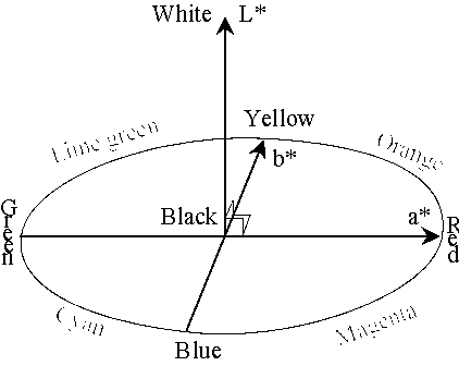
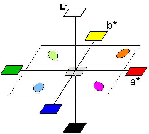
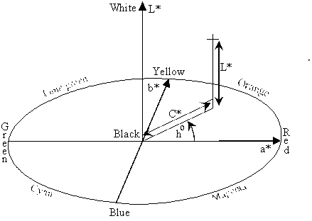
Figure 1: The arrangement of CIE L* a* b* colour space |
|
|
© James H Nobbs |
|
|
|
|
Introduction
It is possible to propose a set of properties for a practical colour space. For example, we can start by considering the co-ordinate system.
|
|
A three-dimensional space in which all surface colours can be represented. |
|
|
A Cartesian set of three axes, each axis direction being perpendicular to the other two. |
|
|
The axes should be chosen to represent parameters that have direct interpretation in visual terms. |
|
|
The distance between points representing the colours of two samples is proportional the visual difference in colour between the samples. |
|
|
The axes are scaled so that a just perceptible colour difference is represented by unit distance. |
A number of colour space systems were developed following the establishment of the CIE XYZ system in 1931. These spaces are of research interest, for practical day to day application the CIE L* a* b* system has become the accepted method of representing the appearance of surface colours . CIE L*a*b* colour space is based on the opponent theory of colour vision.
Psychological primaries
Hering pointed out that we normally describe a colour in terms of four unique hues
|
|
Red, Yellow, Green and Blue. |
All other hues may be described in terms of one or two terms drawn from these four. For example orange is a not a unique hue since it can be described as a reddish yellow, in a similar way purple is not unique since it can be described as a reddish blue. The hues red, yellow green and blue are unique as they cannot be described in any other terms.
Opponent pairs
The four unique hues of red, green, yellow and blue, when taken together with white and black form, a group of six basic colour properties. Red and green are not only unique hues but are also psychologically opponent colour sensations. A colour will never be described as having both the properties of redness and greenness at the same time, there is no such colour as reddish green. In the same way yellow and blue are an opponent pair of colour perceptions.
The six properties can be grouped into three pairs, white/black, red/green and yellow/blue.
CIE L*a*b*(1976) colour space
It seems sensible to associate these three opponent pairs with the three axes of a colour space. On a colour chart, the amount of redness or greenness of a colour could be represented by the distance along a single axis, with pure red lying at one extremity and pure green lying at the other. In a similar way yellow and blue are opposite extremities of a second axis which could be placed perpendicular to the red/green direction. The third axis would go from white to black and lie in the plane normal to the other two.
This is similar to the arrangement of the CIE L*a*b*(1976) colour space which uses three terms L*, a* and b* to represent the opponent signals. The system was defined by the CIE in 1976 as
|
|
L* |
The vertical axis, represents lightness, 100 represents a perfect white sample and 0 a perfect black. |
|
|
a* |
The axis in the plane normal to L*, represents the redness-greenness quality of the colour. Positive values denote redness and negative values denote greenness. |
|
|
b* |
The axis normal to both L* and a*, represents the yellowness-blueness quality of the colour. Positive values denote yellowness and negative values denote blueness. |
The system is illustrated in Figure 1.
|
|
|
|
Figure 1: The arrangement of CIE L* a* b* colour space |
|
The CIE XYZ system was defined so that the Y tristimulus value gives all the necessary information concerning the relative luminosity of a surface. It can be anticipated that the lightness attribute will depend only on the Y tristimulus value. A transformation is needed to convert the Y tristimulus value into a visually uniform scale of lightness.
The form of the transformation equations was obtained from measurement of the Munsell Grey Scale, part of the Munsell Colour Order System. The term Munsell Value is used to denote the lightness of the colour chip and has a range from 10 for a perfect white to 0 for a perfect black. In practice, the grey scale points between 1 and 9 can be made as sample panels. During the development of the scale, the panels at each scale point were adjusted until observers judged them to be equally spaced in lightness from their neighbours.
Measurement of the grey scale showed that the Munsell Value assigned to the chips is uniquely related to their Y value and the relationship could be approximated by a cube root function.
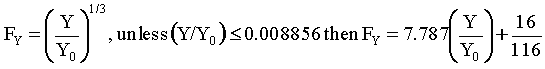
A cube root function is used to form a visually uniform parameter FY from the Y tristimulus value.
|
Equation 1 |
|
Where Yo, is the tristimulus value of a perfect white sample under the chosen illuminant. The ratio Y/Yo is the ratio of the luminance of the surface to the luminance of a perfect white surface viewed under the same conditions of illumination. The ratio takes into account the relative nature of colour vision when judging the lightness attribute of a surface colour.
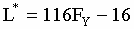
The equation that links L* to FY is obtained by adjusting the scaling to give a range of 0 to 100.
|
Equation 2 |
|
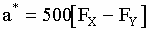
The simplest suggestion is to subtract the red and green tristimulus values to obtain the a* opponent signal.
|
Equation 3 |
|
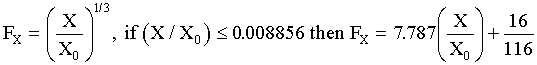
Again however, a transformation to a visual scale is needed before the red and green signals can be subtracted. The cube root function used for the transformation of Y to FY is also used to obtain FX, the visually uniform red signal.
|
Equation 4 |
|
Where Xo is the tristimulus value of a perfect white sample under the chosen illuminant. The opponent value a* is obtained by subtracting FY from FX and multiplying the remainder by a scaling factor. In this way 1 unit distance on the a* scale represents an equivalent visual difference to 1 unit distance along the lightness axis (L*).
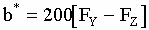
The b* values are obtained by subtraction of the blue from the green signals. Scaling factors are used to ensure that 1 unit distance represents the same visual difference along each axis.
|
Equation 5 |
|
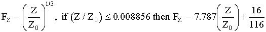
The blue visual signal FZ is obtained using the equation
|
Equation 6 |
|
Where Zo is the tristimulus value of a perfect white sample under the chosen illuminant.
|
|
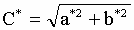
|
Neutral grey samples would have C* values less than 3 units. Whether the surface appears to be weak, medium or intensely coloured depends on both the chroma and the lightness.
A very rough guide to interpretation is
|
|
C* > 0.7 L* |
the surface appears to be strongly coloured |
|
|
C* > 0.3 L* and c* < 0.6 L* |
the surface appears to be of medium intensity of colour |
|
|
C* < 0.2 L* and C* > 3 |
the surface appears to be weakly coloured |
|
|
C* < 3 |
the surface appears to be uncoloured |
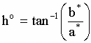
The hue of the surface is indicated by the location of the point in the a* b* plane. The hue angle is the angle, in degrees, between the a* axis and the line joining the point to the L* axis (Figure 2). The hue angle is always measured anti-clockwise from the positive a* axis and is always positive.
|
|
h° hue angle |
|
Pure yellow, green and blue hues
It is traditional to associate one of the psychological primary hues with each axis direction, as shown in the Figures. In reality, the angles of the pure hues do not lie exactly along the axis directions. The true positions of the pure hues are shown in Table 1.
|
|
Table 1: The directions of the psychological
primary hues in
|
||
|
|
Hue name |
h° of associated axis |
h° of pure colour |
|
|
Red |
0 (or 360) |
27 |
|
|
Yellow |
90 |
95 |
|
|
Green |
180 |
163 |
|
|
Blue |
270 |
261 |
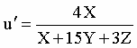
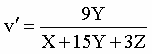
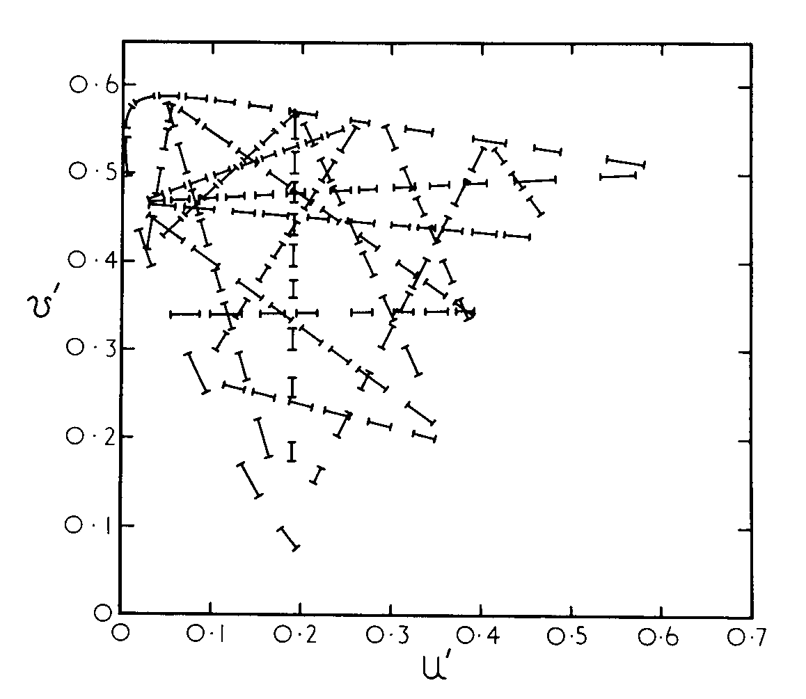
In an attempt to create a more uniform chromaticity diagram, the following equations were used to derive new chromaticity co-ordinates u', v' from X and Y and Z:
|
|
|
|
The resulting chromaticity diagram is shown in Figure 3, with lines whose length shows distances representing equal visual colour differences.
As mentioned previously, a full colour specification must also include a measure of the luminance. In the XYZ system, this was the Y value; however, Y varies in a non-linear fashion with perceived lightness. |
|
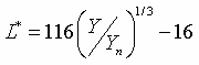
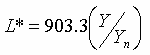
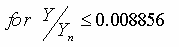
A more linear function, the lightness term L* that is used in the L*a*b* system, was used:
|
|
|
|
|
|
Where Yn is the Y value of the reference white. In the case of reflective colours, the reference white is generally taken to be a perfect reflecting diffuser; for self-luminous displays, the reference white is often taken as an area within the image perceived to be white.
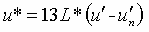
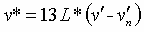
The combination of this approximately uniform lightness scale and chromaticity diagram gives the L*u*v* colour space. This is a three-dimensional space formed by plotting L* on the vertical axis and u* and v* on perpendicular axes in the horizontal plane, where:
|
|
|
|
Where |
|
are the values of u', v' for the reference white. |
L*u*v* space, although approximately uniform, is rarely used for surface colours. It is generally used in the specification of colour displays, where the ease of finding additive mixtures and displaying a colour gamut is useful.
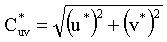
There is a chroma parameter associated with CIE L*u*v* which is determined from
|
|
|
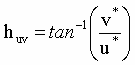
A hue angle is also defined
|
|
|
|
|
|
|
© James H Nobbs |